Interpretable Aeroelastic Models for Control at Insect Scale

Michelle Hickner discusses a new paper in the AIAA journal on Data-Driven Unsteady Aeroelastic Modeling for Control. The study focuses on predicting coefficients of lift and wing deformation for a flexible wing, creating an interpretable, low-rank, linear model for control purposes. The research includes examples of control applications. The motivation behind this work is the interest in insect flight and flight for insect-scale robots, where significant wing deformation is a factor. A rigid model is insufficient for these scenarios, and controlling deformation is crucial, especially considering viscosity at small scales.

Some of our classical models need adjustments. Let's discuss thin airfoil theory, which is the most basic version. It involves an angle of attack, which is the pitch of the wing or plate against the flow.

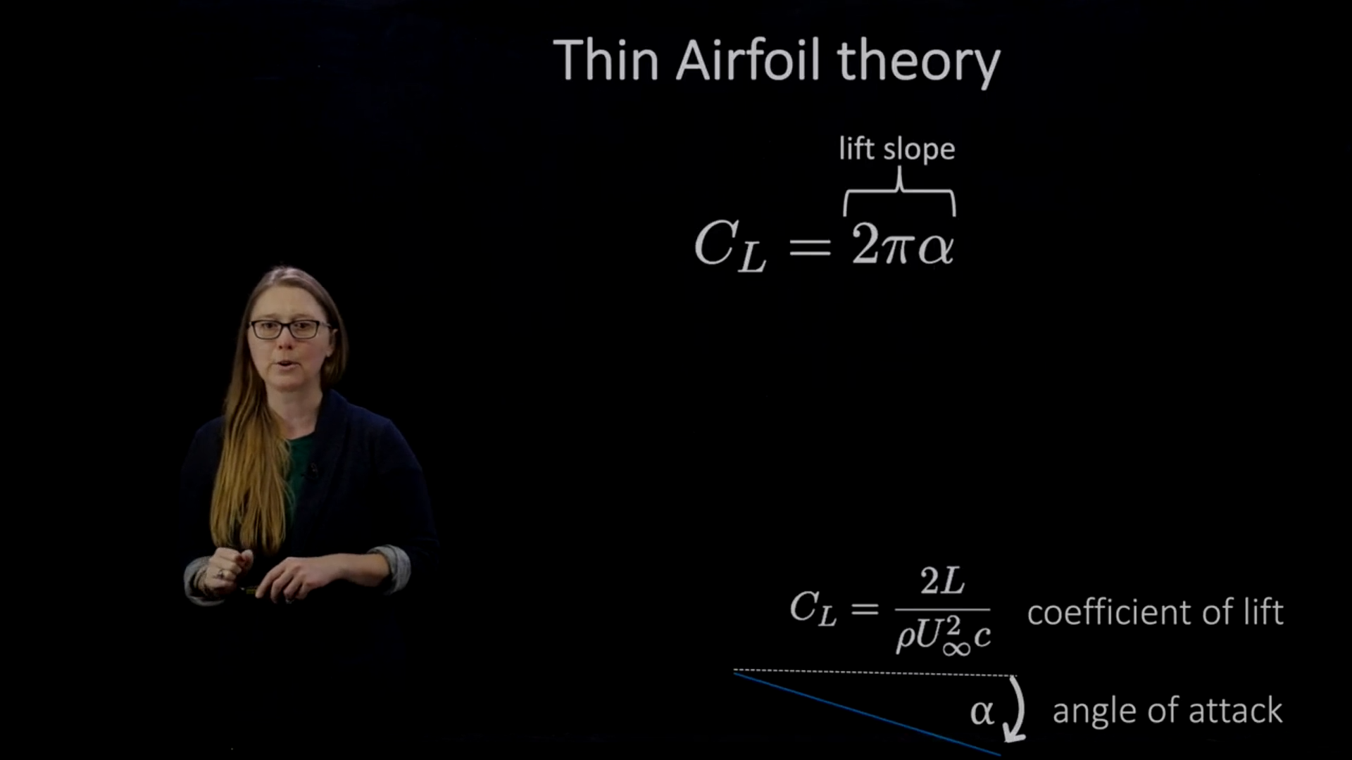
The coefficient of lift is a non-dimensional way of measuring lift force. According to thin airfoil theory, the coefficient of lift is calculated as two times π multiplied by the angle of attack. However, this simple formula is not suitable for all cases. Theodore's model, developed in the 1930s, offers a more comprehensive approach to predicting the coefficient of lift.

In Theodore's model, the two times π lift slope is still present, but it is adjusted for the pitch point, denoted as A in the equation. Additional terms related to added mass, angular velocity, and angular acceleration are included to account for the effects of pitching motions on the lift force. When a structure accelerates through a fluid, it can bring some of the fluid with it, resulting in added mass that must be considered in the analysis.

The model also introduces a term denoted as C of K, which represents Theodore's transfer function. This function, composed of vessel functions, captures the wake vorticity and its impact on lift force. The model is specifically designed for sinusoidal pitching wing motions, with K representing the reduced frequency of the motion. The C of K term indicates how the lift force is affected by the flapping frequency and wake vorticity.

While Theodore's model is useful, it has limitations. The two times π lift slope is primarily applicable to inviscid flow, which may not accurately represent the conditions of insects or robotic flying devices. Additionally, the model is designed for idealized planar wake and sinusoidal motions, making it less suitable for analyzing arbitrary wing motions.

We have flexible wings that have limitations based on their flexibility. The concept of viscosity is important in understanding this. The Reynolds number axis represents the level of importance of viscosity. For larger and faster objects, viscosity may not be significant, such as a whale. However, for smaller objects like insects or insect robots, viscosity becomes more relevant. The Reynolds number axis reflects this change in importance.

The model we are discussing involves predicting the coefficient of lift and curvature. The curvature is our way of measuring deformation, which could also be strain or an angle. We have interpretable coefficients in the model that we will discuss.

The orange term in the model represents the quasi steady term, which is associated with the coefficient of lift. This term changes as we move from a relatively inviscid regime to a viscous regime. The added mass terms in the model have coefficients associated with angular acceleration and angular velocity, which will also be adjusted for the viscous regime based on data from our system.

The model matrix has two rows, one for coefficients associated with the coefficient of lift and the other for coefficients associated with the measure of deformation. The Theodor transfer function includes wake vorticity and bending transients to account for deformation in addition to the coefficient of lift.

To obtain these coefficients, we perform a straightforward procedure involving addition and multiplication. We start by isolating the added mass terms and then conduct a maneuver involving a short pitch up and angle of attack to gather time series data for coefficient of lift and curvature. Peaks in angular acceleration and velocity during this maneuver help determine the coefficients associated with these variables.

The coefficients for angular acceleration and velocity are obtained from the points of maximum acceleration and velocity in the time series data. The quasi steady coefficient is determined from data at the end of the time series when the system has stabilized. This coefficient is crucial for ensuring the model is quasi steady.

We will use an Eigen systems realization algorithm to obtain the A matrix, B matrix, and C matrix that capture all transients and wake vorticity. This includes bending and shedding of vortices. If you are not familiar with Eigen systems realization algorithm, I recommend watching Steve Bruton's videos. More details on building this model can be found in our paper.

To choose the model rank, we need to select the number of latent states X in our model. The goal is to have as few states as possible for fast real-time control. This means being able to predict system behavior as quickly as it occurs. For example, if we are simulating a large CFD with millions of nodes, we want to reduce this to just a few nodes. One approach is to choose from the Hinkel singular values, similar to selecting singular value cutoffs in other systems. It is important to find a balance, as adding more states may result in diminishing returns. Additionally, using a test maneuver can help identify errors and provide insight into system behavior.

When I cut off states, I can better understand what's happening in the system. A dotted black line represents reality, our full-scale model that we are comparing our data to. However, a different maneuver is hidden in the background. The deformation is easier to see in this maneuver, with a dark red line capturing low-rank behavior but not bending or wake vorticity.

The rank four model is not capturing all the necessary elements, as shown by the blue line. The rank six model is looking okay for coefficient of lift, but it is important to include deformation in the model to identify missing elements. Moving to rank eight, we are not perfectly tracking our full order model but are doing a good enough job for feedback control to handle remaining errors.

Interpreting the coefficients from the model is crucial. The test maneuver of pitching up, holding, and pitching down helps us observe acceleration and quasi-steady behavior. Different test maneuvers may be used in various situations. The rank nine model is tracking the data well.

The coefficient of lift and curvature are shown in the model, with good accuracy in rank eight and nine. It is important to consider the interpretation of the data and how it can be used in different scenarios.

I have separated the upper curve into individual contributions from angle of attack, angular velocity, angular acceleration, and remaining transients and bending in the C matrix. The coefficients of lift show that all of these contributions are important in deformation. The speed bump curve represents the contribution to deformation from angle of attack, while the green curve represents bending modes and transients, which are also significant. This information will be useful for designing control objectives, as deformation mainly tracks angle of attack rather than acceleration. This unexpected result will help us in utilizing this data effectively.

Here are some examples of Control architecture. We will be using a full order model to account for all nonlinearity, but for feedback prediction, we will use a linear rank nine model. This linear state space low rank model will be utilized in model predictive Control, as shown in the purple box. Constraints on curvature will be applied to prevent excessive bending. Additionally, we will test the system with both curvature constraints and reference values, such as a reference coefficient of lift. The cost function will determine the importance of each parameter.

In this example, we are not considering curvature, only focusing on lift. The light gray background serves as our reference. The coefficient of lift is tracking well, but curvature changes slowly and can lead to vibrations that lower service life.

A green curve has been added to the plot we previously viewed. This curve represents the reference curvature, indicating that the curvature will approach zero after completing the maneuver. The trade-off made considers both curvature sum and lift sum. As a result, the lift tracking has slightly worsened. However, the vibrations in the curvature tracking have been reduced more quickly. This trade-off may be beneficial for extending the service life, even if it results in slightly bumpier lift.

Having an interpretable model helps us avoid undesirable situations, such as the yellow and red curves shown here. This test maneuver involves pitching up and holding pitch down at various speeds to assess the quasi-steady contribution. If the speed is too high, the coefficient of lift cannot accurately track the reference (light gray curve). The yellow curve falls short of reaching the reference, which is a common occurrence. However, the orange curve, when performed at a slightly slower speed, successfully tracks the reference. A constraint on curvature has been applied to prevent excessive stress on the leading edge, which could lead to breakage. Increasing the angle of attack while imposing this constraint is necessary to achieve the desired outcome.

The longer the higher coefficient of lift needs to be maintained, the more the angle of attack must be increased. Short maneuvers rely on angular acceleration, while longer maneuvers require a gradual increase in pitch. The interpretable coefficients indicate that deformation closely follows the angle of attack. Control objectives should focus on accelerating using angular acceleration rather than simply maintaining higher angles of attack. These test maneuvers demonstrate this concept, but real-world systems can be more complex. Interpretable coefficients allow for quicker planning of controls by providing insight into potential issues and avoiding the need to decipher complex physics.

Interpretable models help us avoid undesirable situations like the yellow and red curves. The test maneuver involves pitching up and holding pitch down at different speeds to measure the quasi-sty contribution. If the speed is too fast, the coefficient of lift cannot track the reference (light gray curve). The yellow curve falls short, while the orange curve tracks it well but with a constraint on curvature to prevent excessive stress. Increasing the angle of attack requires a higher coefficient of lift, which relies on angular acceleration for short maneuvers and pitching up for longer durations.

Interpretable coefficients show that deformation tracks the angle of attack, emphasizing the importance of control objectives that prioritize angular acceleration over maintaining high angles of attack. This approach simplifies control planning by quickly identifying potential issues based on coefficient values. The method discussed involves creating a linear low-rank model for an aeroelastic system with a flexible wing, accurately predicting lift and deformation by leveraging data. For more details, refer to our paper. Thank you for your attention.