On-the-fly clustering for exascale molecular dynamics simulations.

Welcome to the next installment of our Computer Physics Communications Seminar Series. Today, we are pleased to have Alizée Dubois and Thierry Carrard from CEA in France. They will discuss their recent paper on "On-the-Fly Clustering for Exascale Molecular Dynamics Simulations."

Without further delay, I will now turn the presentation over to our speakers.

Good afternoon, everyone. It is a pleasure to be here, and we appreciate the opportunity to present our work on clustering methods for exascale molecular dynamics simulations. We are part of a laboratory located in Bruyères-le-Châtel, south of Paris, where we focus on studying matter under extreme conditions.

In extreme conditions, we aim to understand how the physical properties of matter are altered under shock conditions. This includes examining the equation of state, which describes pressure as a function of density, and investigating phase transition mechanisms, such as transitions between solid, liquid, and plasma states. We also analyze how shocks can induce damage and how the constitutive behavior of solid materials is affected.

Extreme conditions involve very high pressure applied over a very short time scale or at a very high loading rate. To achieve these conditions, we utilize various loading devices. For instance, we employ diamond anvil cells for generating super high pressures in the hundreds of gigapascals, albeit at relatively low loading rates. For higher loading rates, we utilize gun techniques.

In extreme conditions, we aim to understand how the physical properties of matter are altered under shock conditions. This includes examining the equation of state, which relates pressure to density, as well as the mechanisms of phase transitions, such as solid to solid, solid to liquid, or solid to plasma. We also investigate how shocks can induce damage and affect the constitutive behavior of solid materials.

Extreme conditions are characterized by very high pressure applied over a very short time scale or at a very high loading rate. To achieve this, we utilize various loading devices. For instance, a diamond anvil cell can generate super high pressures, reaching hundreds of gigapascals, but at relatively low loading rates. For higher loading rates, we employ a gas gun, which propels a bullet that impacts a target, generating a shock wave.

Additionally, we use lasers that focus energy onto a metal surface, creating a plasma that ejects material and generates shock waves in the sample. A shock wave is defined as a compressive pressure wave that propagates through the material.

A pressurized chamber can deliver high-pressure gas onto a bullet, which then impacts the target and generates a shock wave. Additionally, a laser can be used to focus on the metal, creating a plasma that ejects material and produces shockwaves in the sample.

A shock wave is a compressive pressure that propagates through a medium. It can reflect off free surfaces, leading to tension loading. However, materials do not sustain tension loading for extended periods; instead, they may nucleate bubbles and generate ejecta, as demonstrated in the accompanying video.

In this seminar, we aim to analyze phenomena such as bubble generation, ejecta formation, and void creation.

We aim to understand the implications of voids and bubbles at both the atomic and grain scales. The slide presents a monocrystal of Tantalum, along with an image of Tantalum grains at a higher magnification, and the surface of a sample impacted by a laser, which illustrates the void generation.

To analyze these phenomena, we utilize several computational tools. For the atomic scale, we employ Molecular Dynamics simulations. At the intermediate scale, we use continuum mechanics codes, and for the structural scale, we apply hydrodynamics codes. This presentation will primarily focus on an example using our Molecular Dynamics code.

Hello everyone. I am Cheria, responsible for overseeing our computer science initiatives, particularly in simulation tools. Our journey began with the development of our Molecular Dynamics code, ExaMD, with a strong emphasis on high-performance computing facilities. Over the years, we have refined this tool and introduced numerous massively parallel algorithms, including GPU ports for most of these algorithms. This advancement has sparked interest in optimizing other simulation tools to leverage similar parallel algorithms tailored for specific simulations.

For example, we have created a specialized N-body simulation platform called Exabody. This platform serves as a foundation for any N-body based simulation code. Currently, we have three simulation codes built on Exabody that model various systems, including small grains of matter, rigid bodies like sand grains or powders, and complex rigid bodies that incorporate contact dynamics, friction, and collision detection.

In addition to our work with Molecular Dynamics, we are also exploring hydrodynamics through particle-based simulations using Smooth Particle Hydrodynamics. This approach is particularly advantageous for scenarios where traditional mesh-based methods are insufficient.

Hello everyone. I am Cheria, and I oversee the computational aspects of our projects, particularly in simulation tools. Our journey began with the development of our Molecular Dynamics code, ExaMD, which emphasizes high-performance computing capabilities. Over the years, we have created numerous massively parallel algorithms and GPU ports for most of these algorithms. This advancement has sparked interest in optimizing other simulation tools to leverage similar parallel algorithms tailored for specific simulations.

Currently, we have established a specialized N-body platform called ExaNBody. This platform serves as a foundation for any N-body simulation code. To date, we have developed three simulation codes based on ExaNBody, which can simulate various systems, including small grains of matter, rigid bodies such as sand or powders, and more complex interactions involving rigid bodies with contact dynamics, friction, and collision detection. In addition to our Molecular Dynamics code, we are also exploring hydrodynamics through particle simulation techniques, specifically smooth particle hydrodynamics, which address the limitations of mesh-based methods.

We have created a robust ecosystem for developing our simulation software tailored for high-performance computing. This ecosystem consists of three main components. First, we utilize industry-standard low-level libraries, including MPI, OpenMP, C++, YAML for user inputs, and CUDA and HIP for GPU acceleration. Built on top of these low-level standards, we have developed three software layers. The first is OnikaBrick, which serves as the interface with the hardware and incorporates a component-based programming model. The second layer is ExaNBody, which focuses on N-body parallel algorithms, and on top of this, we have our three simulation code applications.

We have developed a comprehensive ecosystem for our simulation code software tailored for high-performance computing facilities. This ecosystem consists of three primary components.

First, we utilize industry-standard low-level libraries, including MPI, OpenMP, C++, YAML for user inputs, and CUDA and HIP for GPU acceleration. These libraries form the foundational layer of our software.

Building on this foundation, we have created three proprietary software layers. The first is Onika Brick, which serves as the interface with the hardware and supports a component-based programming model. The second is exaNBody, which focuses on N-body parallel algorithms. Finally, our three simulation code applications are built on top of these layers.

The accompanying slide illustrates two of our simulation codes. At the top, there is an example of a block of matter subjected to shock from a piston, resulting in rapid movement and the ejection of micro jets of matter through molecular dynamics. The bottom section depicts a rotating drum containing millions of small grains of material. As the drum rotates, the grains mix and move dynamically. Now, let us focus on the molecular dynamics aspect of our work.

The primary focus of Molecular Dynamics is its nature as an unbound problem characterized by specific properties. It employs a potential function that describes the interactions between particles, indicating whether they are repelling or attracting each other. When particles are in close proximity, they repel each other, while at greater distances, they exhibit attractive forces.

A key feature of this potential function is its rapid convergence towards zero. To effectively manage these interactions, Molecular Dynamics utilizes a cutoff approach, limiting the consideration of particle interactions to a defined maximum radius. This ensures that, at any given moment, only particles within a specified distance from a central particle are taken into account.

Molecular Dynamics is characterized as an unbound problem, yet it possesses strong properties. The potential function defines the interactions between particles, indicating that they repel each other when too close and attract as they move further apart. A key feature of this function is its rapid convergence towards zero.

To optimize calculations in molecular dynamics, we implement a cutoff, limiting the potential function to a maximum radius. This approach ensures that we only consider particles within a specified distance from a central particle at any given moment.

In the context of parallelization, we utilize a domain decomposition strategy. Each computation node has a shared memory horizon, and each MPI process operates within a designated bluish area, surrounded by a ghost region. This ghost area contains copies of particles from neighboring MPI processes, facilitating the exchange of information necessary to update properties across processes.

Now, we will apply the molecular dynamics codes to perform physics simulations. For instance, we can observe a video illustrating an impact on Taluma, showcasing the impact event, the reflection of waves, and the nucleation of voids.

The simulation involves 83 million atoms, and our objective is to analyze the resulting data effectively. We aim to detect voids, as well as determine their positions, growth velocities, and volume ratios. However, existing literature offers limited methodologies for this analysis.

One notable tool in the field is the VET code, which provides extensive post-processing capabilities. Despite its strengths, it is only parallelized using OpenMP, which constrains its performance based on the system architecture. As a result, when processing tens of millions of atoms, the tool becomes inefficient. Additionally, since VET is a post-processing tool, it requires the recording of vast amounts of data to achieve high temporal resolution, making it unsuitable for our specific analysis needs.

We propose a new on-the-fly approach for developing an algorithm that detects particle aggregates or, more broadly, regions of interest within molecular dynamics simulations. This algorithm should be versatile, capable of identifying any binarizable zone of interest. It must also be robust and scalable to function effectively with billions of atoms. Additionally, it should be simple and low-cost relative to the overall simulation expenses. This will enable physicists to obtain accurate measurements, including quantification of bars and qualification of data. To achieve these objectives, we have selected connected component analysis as our methodology.

We propose a new approach for on-the-fly detection of particle aggregates and regions of interest within molecular dynamics simulations. This algorithm must be versatile, capable of identifying any binarizable zone of interest. It should be robust and scalable to handle simulations involving billions of atoms. Additionally, it should be cost-effective relative to the overall simulation expenses, enabling physicists to obtain real measurements, including quantification of bars and qualification of data. To achieve these objectives, we have selected connected components analysis.

Connected components analysis can be divided into two main branches: one developed by the image processing community and the other by the graph processing community. The image processing community typically employs shared memory algorithms with a finite number of passes, which are not scalable beyond a single node. Therefore, utilizing these algorithms requires integration into a routine memory system. Conversely, the graph processing community offers fully parallelized algorithms, although many are iterative and would need adaptation for 3D images.

The reason for focusing on images is that we work with atomic data, specifically the movement of atoms. However, we will not remain solely on atomic data; instead, we will project our atomic quantities onto a regular grid. This approach will allow us to define our spatial subdomain effectively.

Connected components analysis can be categorized into two primary branches: those developed by the image processing community and those from the graph processing community.

The image processing community primarily utilizes shared memory algorithms that operate with a finite number of passes, which limits their scalability to a single node. To effectively employ these algorithms, it is necessary to integrate them into a structured memory system.

In contrast, the graph processing community has developed algorithms that are fully parallelized and typically involve many iterative processes. However, these algorithms require adaptation for application to 3D images.

The emphasis on images arises from the need to work with atomic data, which consists of moving atoms. However, our focus will shift from atomic data to projecting these quantities onto a regular grid. This involves subdividing the spatial domain into cells, allowing us to define subcells or box cells for our analysis. Each atomic quantity will be projected onto these boxes, resulting in a 3D voxelized image. Our initial approach will be to implement the methodologies from the image processing community.

The analysis begins by subdividing the space into cells, which allows us to define subcells or box cells. Each atomic quantity is projected onto these boxes, resulting in a 3D voxelized image. Our initial approach will be to implement the image processing methodology developed by the COMMUNITY, as it aligns closely with our existing data format.

This work is based on the PhD thesis of Kan, who conducted the foundational research. I am here to present his findings and provide a comprehensive overview of the work he has accomplished.

The algorithm begins with the projection step, transitioning from atomic data to cell representation. Following this, we will conduct connected component labeling and perform subsequent analysis. The process involves moving from atomic values to binarized quantities, and then to aggregation.

The algorithm begins with a projection step, transitioning from atomic data to a cell-based representation. Following this, we will perform connected component labeling and analysis. This process involves moving from atom-based quantities to binarized data and then to aggregation.

The projection steps are designed to enhance the distribution of the quantities. Key parameters for the projection include the atomic projection splat, which serves as a smoothing parameter for the fields, and the size of the simulation subcell, which dictates our discretization approach.

After projecting the atomic quantities—such as density, velocity, or any mechanical field computed per atom—we obtain a visual representation of these fields. At this stage, we will establish a generalization threshold. For instance, when considering density, we have various threshold options. A stringent criterion may require selected voxels to be entirely void, while a more lenient approach allows for some flexibility. The choice of threshold will influence the detection of void quantities, particularly in circular structures.

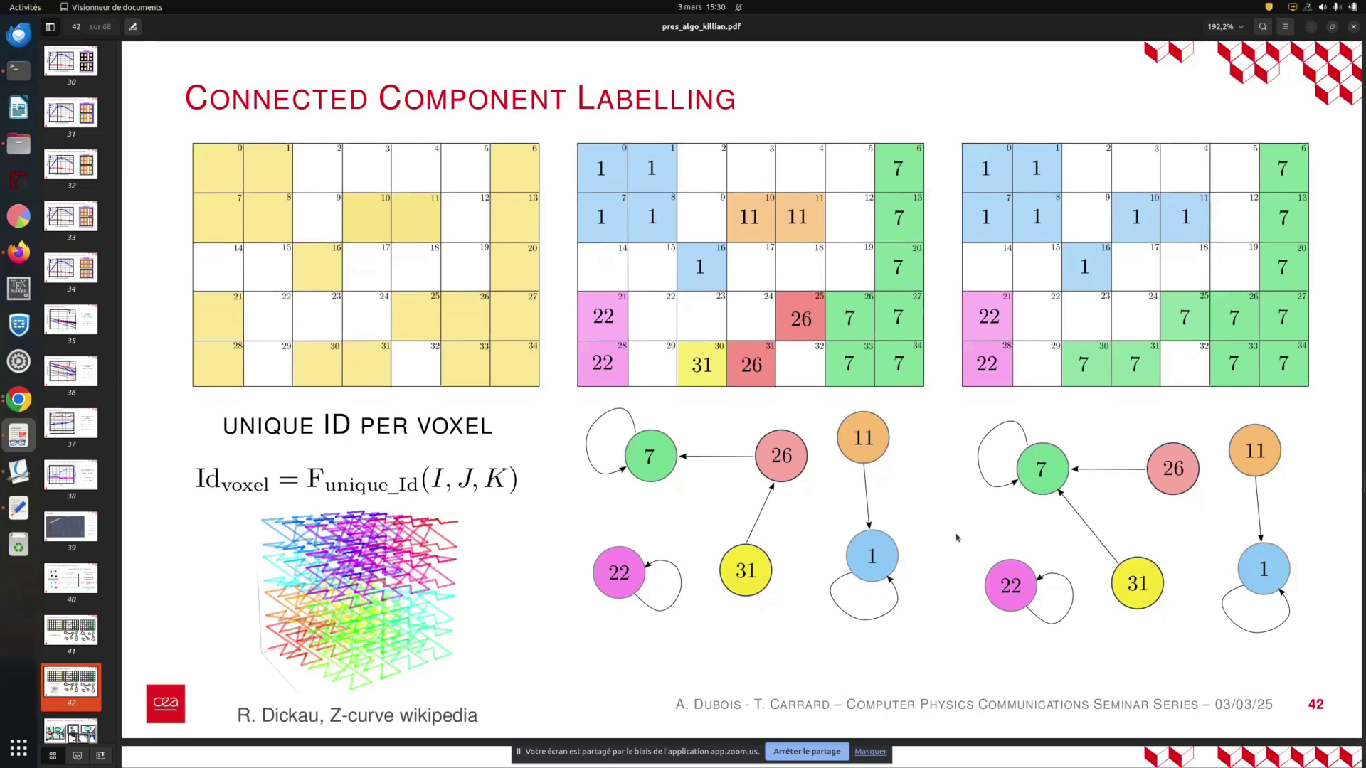
Once the projection is complete, we will have a visualized image annotated with unique ID labels for each cell, ranging from 0 to 5. These IDs correspond to the cells' positions within the global simulation, providing a convenient reference that will be utilized in subsequent analyses.

In this process, we begin by assigning unique identifiers to each voxel in the simulation. As we traverse through the voxels, we label the first voxel as 1. The second voxel, which is connected to the first, receives the same label. This continues sequentially until we reach the sixth voxel, which is isolated. At this point, we define a new connected component and increment the label for the next set of connected voxels.

As we progress to the next row, we find that the sixth voxel is connected to one of the previously labeled voxels. We can then assign it the same label as the first connected component. This process allows us to establish a global graph of connected components. However, not all voxels are yet connected, necessitating a final pass to consolidate the information and assign labels based on the minimum identifiers.

The objective is to achieve domain labeling, which is necessary for parallel processing between threads and MPI (Message Passing Interface). The domain labeling between threads is relatively straightforward, but we will focus on the more complex MPI domain labeling next.

You begin with your unique voxel idea and proceed to label each voxel. Start with the first voxel, labeled as 0, and assign it the label 1. Continue this process for the second, third, fourth, fifth, and sixth voxels. The sixth voxel is isolated and currently unconnected, prompting the definition of a new connected component or level.

Next, move to the second line. The sixth voxel is now connected to a voxel from the first level, allowing you to assign it the same label. This process facilitates the creation of global graphs. However, at this stage, not all voxels are interconnected, necessitating a final pass to consolidate the information and unify all levels to the minimum label assigned.

The objective is to achieve DOMAIN labeling, which involves the interaction between threads and MPI. The DOMAIN labeling between threads is relatively straightforward. We will now focus on the more complex MPI DOMAIN labeling.

To implement this, we will utilize a master MPI to facilitate the stitching process. Each MPI will send messages to the master MPI, enabling it to perform the global connection. For illustration, consider a scenario with one MPI and one NKI, where the local graphs are constructed by the NPI, as shown on the right.

In this process, we utilize a master MPI to facilitate the stitching of data. Each MPI sends messages to the master MPI, enabling it to establish global connections.

Consider the scenario with one MPI and one NKI. The local graphs constructed by the NPI are displayed on the right. For the 36 labels, we observe connections to subsequent labels. Each MPI performs local connected component labeling (CCL) at the boundaries of its regions, utilizing the concept of ghost layers.

At the boundary of each MPI, such as the boundary of MIN, there exists a ghost layer comprising the first layer of voxels outside the MPI domain. This allows for the execution of local 2D CCL across these two layers of voxels. For instance, MIN will send a message to the master MPI, reporting the IDs of the voxels outside its spatial zone and those within it. If label 36 is connected to label 25, MIN will communicate this as "36 25," recognizing that label 25 is also connected to label 3, thus reporting the root of the connected component.

The same process applies to label 39, which connects to 25, and subsequently, the connections continue with 25 to 43. This pattern allows for the aggregation of connections, such as 25, 36, and 362. Each MPI sends its local CCL information at the boundaries to the master MPI, which consolidates this data and transmits a unified message back to each MPI.

The connection between the 36 labels and the second label is established through the graph created by the MPI. Each MPI will perform local connected component labeling (CCL) at the boundaries of its regions, utilizing the concept of ghost layers. A ghost layer is the first layer of voxels outside the MPI domain, which allows for local 2D CCL to be executed between these layers.

For instance, at the boundary of MPI MIN, it will send a message to the master MPI that includes the identifiers of the connected cells both inside and outside its spatial zone. If the label 36 is connected to label 25, MPI MIN will report this connection as "36-25." It also recognizes that label 25 is connected to label 3, thus reporting the root of the connected component. This process is repeated for other labels, such as 39 reporting "39-25" and then "25-43."

Subsequently, the master MPI consolidates this information from all MPIs, reducing it to a single message that reflects the global connection. This allows for the local graphs of each MPI to be summarized effectively.

In summary, the algorithm involves multiple steps where all workers are engaged in processing. The left side of the slide outlines these steps, while the right side presents a graph indicating the number of active workers and their respective timeframes. Initially, all workers are operational; however, a bottleneck may occur during the information reduction phase at the boundaries, potentially leading to traffic congestion in the MPI system. It is crucial to assess whether this presents a problem for the scalability of our algorithm.

To evaluate the performance of our algorithm, we conducted a simulation involving 81.9 million atoms. The accompanying graph illustrates the work ID, representing the number of cores, while the color-coded activity on the cores is displayed over time. The lower graph integrates this information, showing the number of active workers over time.

We observed a bottleneck caused by the information reduction at the master MPI, which leads to a temporary slowdown. Although this is a drawback, it does not significantly impact the overall analysis time, indicating that it is manageable.

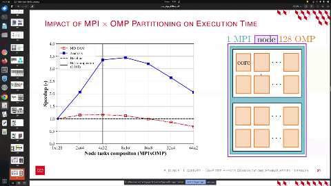
Next, we aim to determine the optimal partitioning time for the NNP, which should enhance the efficiency of the Molecular Dynamics analysis. Our computational nodes consist of 64 cores, and we can explore various decompositions, such as 1 MPI with 125 processes or 2 MPI. However, increasing the number of MPI processes leads to a higher volume of message exchanges. Conversely, increasing the number of threads can result in longer memory access times, making it less optimal.

Ultimately, we seek the best scenario for performance, which we identified as a configuration of 4 MPI with 32 processes, maximizing overall efficiency.

To evaluate the performance of our simulation, we conducted a test involving 81.9 million atoms. The accompanying graph illustrates the activity across the cores over time, with a specific focus on the workload distribution indicated by the work ID. The lower graph integrates this information, showing the number of active workers on the cores throughout the simulation. We observed a bottleneck related to the communication of information through the master MPI; however, the time required for this process is relatively minor compared to the overall analysis duration. While this presents a limitation, it is manageable and not a critical issue.

Our goal is to determine the performance of the algorithm by selecting the optimal partitioning for the Neural Network Potential (NNP). The ideal partitioning should enhance the efficiency of the Molecular Dynamics analysis. We utilize nodes composed of 64 cores each, allowing for various decomposition configurations. For instance, a configuration of 1 MPI with 125 threads can be tested. Increasing the number of MPI processes results in a higher volume of messages, but adding more threads can lead to increased memory access time, which may not be optimal. Therefore, we aim to identify the best scenario, ultimately determining that a configuration of 4 MPI with 32 threads yields the best performance.

In terms of strong scaling, we maintain a constant load of 81.9 million atoms, which is relatively manageable for our system.

We evaluate the reduction in computation time as we increase the number of calls. The dotted black line represents the ideal scenario. Although we do not perfectly align with this ideal, our performance improves with a higher load of atoms.

In our analysis of weak scaling results, we maintain a constant load per core. As we increase the number of cores, we also increase the number of atoms proportionally. This approach allows us to evaluate the efficiency of our computation under varying workloads. The dotted black line represents the ideal scenario, and while we do not perfectly align with it, we observe that as the number of atoms increases, our performance improves relative to this ideal case.

For the weak scaling results, we maintain a constant load per core. As we increase the number of cores, we also increase the number of atoms, targeting approximately 160,000 atoms per core. Although the scalability of our existing system is not ideal, the scalability of the molecular dynamics is nearly perfect, indicating that communication is not a significant issue.

In our analysis, while the performance is not as strong, the bottleneck we identified—reducing the information from a single molecular interaction—is manageable. Our primary objective is to conduct an analysis that does not excessively increase computation time. We must ensure that the time required for analysis does not exceed that of a single step of molecular dynamics. The accompanying slide presents the ratio of analysis time to one step of dynamics.

To achieve approximately 160 × 10^3 atoms per core, we note that while the scalability of our existing blue system is not ideal, the scalability of molecular dynamics is nearly perfect, and communication issues are minimal. Although our analysis is less efficient, the bottleneck we identified indicates that reducing the information from a single molecular interaction (MI) is manageable.

We aim to ensure that our analysis does not require excessive computational time. It is critical to consider the time associated with molecular dynamics; specifically, the analysis must not exceed the computational cost of a single step of dynamics. The following graph illustrates the ratio of analysis time to one step of molecular dynamics across varying loads and core counts.

The light blue points represent data from low load strength scaling, while the pink points correspond to high loads. The points with varying colors reflect weak scaling. As observed, the load increases with the number of cores. When optimization is adequately implemented, the analysis time approaches 5% of the molecular dynamics time, which is satisfactory. Consequently, this analysis will not be conducted after every step but rather every 10 or 100 steps, making its impact negligible compared to the overall cost of molecular dynamics.

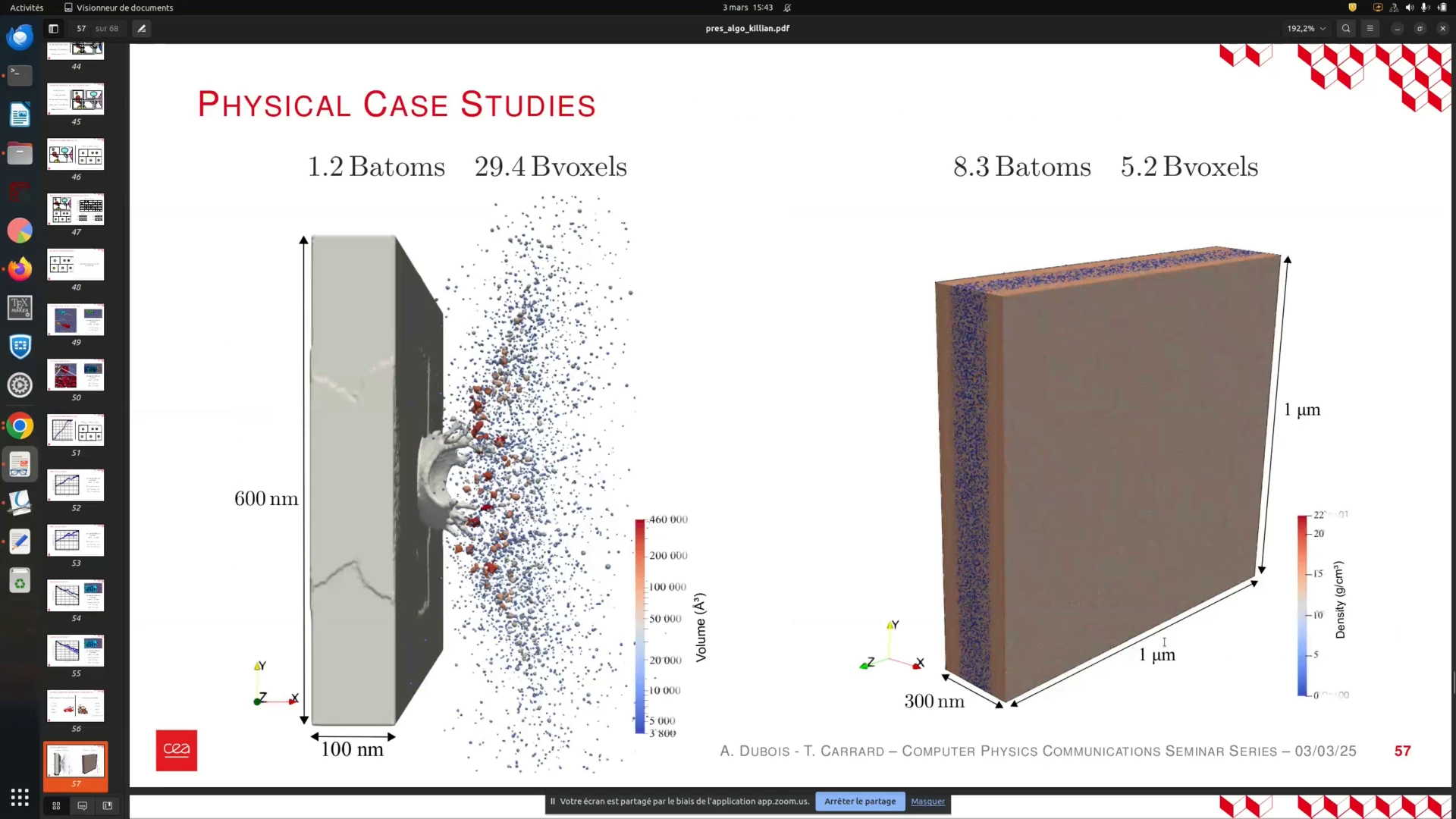
In this section, we present an example comparing a Tantalum structure of 1 micron by 1 micron to one measuring 150 nanometers. This represents a significant advancement in our capabilities. We successfully performed connected components analysis and detected all relevant features, which was a highly satisfactory outcome. Additionally, we will discuss the image processing techniques employed in this analysis.

The image processing method for developing connected components has been established. We will now transition to a new implementation focused on graph processing.

As previously mentioned, the algorithm developed during the PhD is efficient and well-optimized. However, it has a limitation: it consolidates information into a central MPI node. To address this, we aimed to create an alternative algorithm for two main reasons. First, we sought a simpler algorithm that could be adapted for GPU implementation in the near future. Second, for large simulations, we wanted to ensure robustness, avoiding scenarios where all information is gathered on a single node.

The alternative implementation we have recently finalized maintains the same starting point as before. Regarding the local MPI process, it operates similarly to the previous algorithm.

The image processing method for developing connected components is based on the concept of image connected components. We will now shift our focus to a new implementation from a graph processing perspective. As previously mentioned, the algorithm developed during the PhD is efficient and highly optimized. However, it has the limitation of aggregating condensed information to a central MPI node.

To address this, we aimed to create an alternative algorithm for two primary reasons. First, we sought a simpler algorithm that could be easily adapted for GPU implementation in the near future. Second, in cases involving large simulations, we wanted to ensure robustness, avoiding any implementation that centralizes all information on a single node. The alternative implementation has recently been finalized, and I will present it to you now.

The starting point remains the same as before. From the perspective of the local MPI process, our approach is similar to that of the previous algorithm. The key difference lies in the function used to associate a unique Voxel ID with the coordinates of each cell. This function is crucial to the algorithm's effectiveness and must be deterministic, invariant to the number of MPI processes, and exhibit locality features, which is why we employ a curve-based function.

Additionally, it is essential to know the main and maximum possible values for this function in advance, prior to propagating the labels. These properties are significant, and their importance will become clear shortly. We begin with unique IDs assigned to each voxel and then propagate by identifying the minimum label ID within the connected components.

The primary distinction in this process lies in the selection of the function used to associate a unique Voxel ID with the cell coordinates. This function is crucial to the algorithm, as its deterministic nature must remain invariant to the number of MPI processes and incorporate a locality feature. Consequently, we employ a curve-based function. It is essential to identify the main and maximum possible values for this function prior to label propagation, as these properties are significant for the algorithm's effectiveness.

We initiate the process by assigning unique IDs to each voxel and then propagate the minimum label ID within each connected component. Instead of relaying information to a central MPI process, we leverage the existing ghost layer communication algorithm from standard Molecular Dynamics simulations. This approach updates values in the ghost area based on computations from neighboring MPI processes.

Once we receive updated information from neighboring processes, we may encounter additional labels that require further propagation. The process alternates between local steps for propagating the minimum local ID within the connected component of a local MPI process and steps for updating the ghost areas. This iterative method can lead to more iterations, particularly in cases where a connected component spans multiple subdomains. Each time we propagate and reach the ghost area, the neighboring MPI processes will continue the propagation, resulting in a greater number of iterations needed to achieve global stability. This stability is easily identified when updating values from neighboring MPI processes.

After completing a series of iterations to propagate the minimum local ID within each connected component, we utilize the existing ghost layer communication algorithm, similar to that used in standard Molecular Dynamics simulations. This approach updates the values in the ghost areas based on computations from neighboring MPI processes.

Once updated information is received from neighboring processes, we may encounter additional labels or lower minimum IDs that require further propagation. We alternate between local steps, where the minimum local ID is propagated within the MPI process, and steps that update the ghost areas. This process may reveal lower label IDs in the surrounding area that need to be propagated again.

It is important to note that more iterations may be necessary, especially if a connected component spans multiple subdomains. As propagation occurs, each MPI process updates its ghost areas, and these updates are communicated to neighboring processes. This iterative process continues until a global stable state is achieved, which is identified when no changes are observed in the state across all MPI processes during the local minimum propagation step. At this point, further iterations are unnecessary.

In this state, each MPI subdomain represents a part of a connected component. It is essential to aggregate metrics for every connected component, such as the number of voxels and other relevant data. However, we aim to avoid centralizing all information to a single MPI process. Instead, we assign each connected component to a specific process, designated as the owner, responsible for aggregating all values associated with that component.

To facilitate this, we introduce a function G. This function determines the MPI rank of the process responsible for aggregating metrics for each connected component label, based on the voxel ID and the total number of MPI processes.

In this state, each MPI subdomain corresponds to a specific connected component. We must aggregate metrics for every connected component, such as the number of voxels and other relevant metrics, using the information contained in each voxel. Rather than consolidating all this data into a single MPI process, we assign each connected component to a designated owner process responsible for aggregating its metrics. This is achieved by implementing a function ( G ) that, for each connected component label (or voxel ID), determines the MPI rank of the process responsible for aggregation based on the total number of MPI processes.

Each MPI process can deterministically identify the owner of any arbitrary connected component ID. Consequently, if a process holds part of a connected component within its local subdomain, it can accurately determine the amount of information to send to other MPI processes. This is represented in the send count array. Additionally, we can construct a receive code to ascertain how much information needs to be received from other MPI processes. We utilize the MPI All-to-All communication model, allowing each MPI processor to exchange data with other processes, thereby facilitating efficient data transfer after these steps.

Each MPI process is responsible for maintaining the complete information for every connected component it owns. Subsequently, all MPI processes can write the connected component properties in parallel to a result file. It is important to note that throughout the algorithm, there is no step that requires gathering information from all connected components.

This slide presents a detailed overview of the test case utilized in our analysis. Similar to the previous scenario, we examined the algorithm developed by Killian, which represents a worst-case situation characterized by numerous connected components that are sparsely distributed across the domain. This algorithm demonstrates excellent scalability when handling many small connected components that are uniformly distributed throughout the simulation domain.

However, in this instance, we observe a significant connected component that extends widely. This phenomenon occurs due to the presence of numerous filaments that link groups of atoms together, resulting in a more complex structure within the simulation.

This slide presents a detailed examination of the test case utilized. In the previous scenario, we analyzed the algorithm developed by Killian, which represents a worst-case scenario characterized by numerous connected components that are sparsely distributed across the domain. This situation poses a challenge for the algorithm, as it is designed to scale effectively when many small, connected components are uniformly dispersed throughout the simulation domain.

In this particular case, however, we observe a significant connected component that extends widely. This phenomenon occurs due to the presence of numerous filaments that interconnect groups of atoms. Understanding the algorithm's performance in this worst-case scenario is crucial for evaluating its robustness and effectiveness.

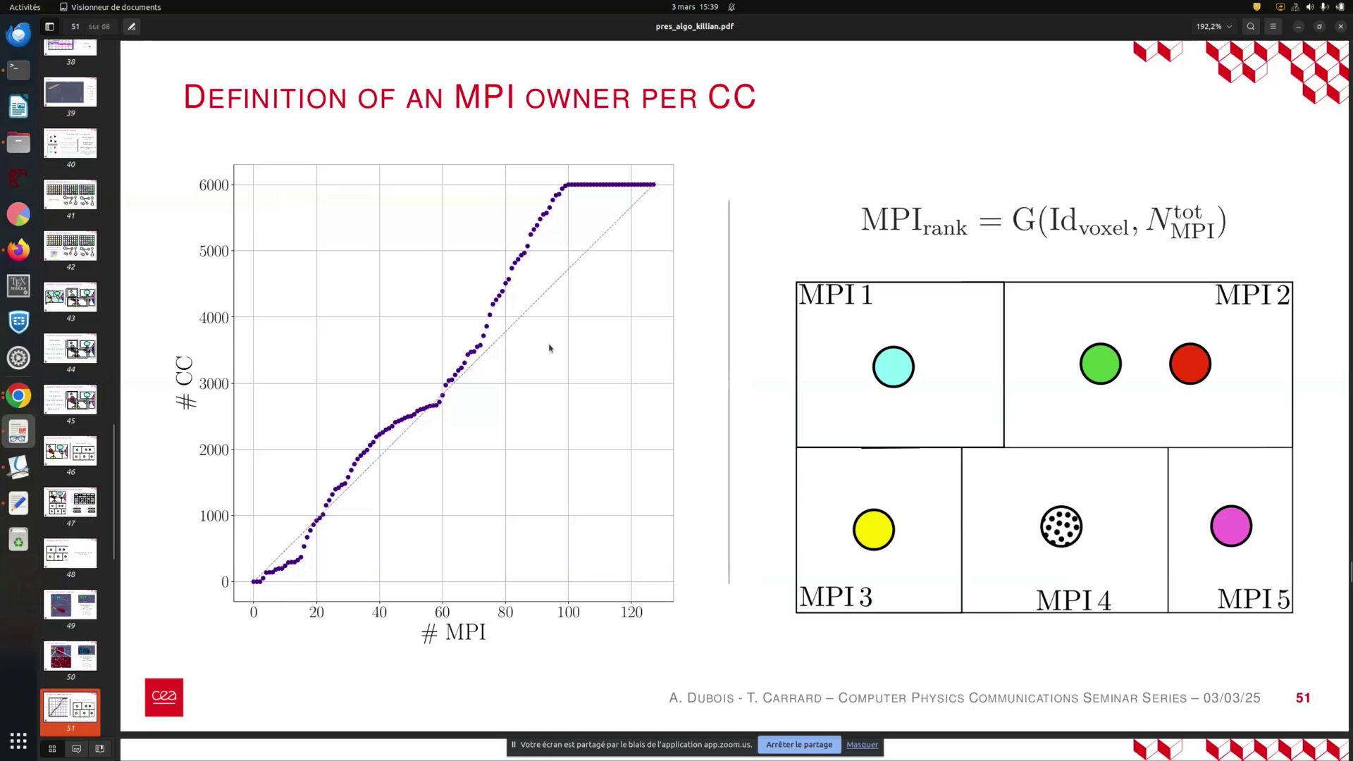
This slide illustrates the distribution of connected components when utilizing a static and deterministic approach. The distribution is based solely on the ID assigned to different MPI processes. As shown, the distribution is not ideal; several MPI processes, particularly those associated with higher values, have few or no connected components.

Despite this, the overall repartition is adequate for our algorithm's scalability, particularly from a memory perspective. This demonstrates that the algorithm can effectively handle both weak and strong scaling scenarios.

This slide illustrates the distribution of connected components within the context of a static and deterministic distribution method, which allocates collected components based solely on their IDs across different MPI processes. The distribution is not optimal; we observe that many MPI processes, particularly those associated with higher values, have few or no connected components. However, this is not entirely detrimental. The repartitioning is sufficient for our algorithm to scale effectively, particularly from a memory perspective.

Regarding weak scaling, our algorithm demonstrates slightly less scalability compared to other algorithms. This is partly due to our focus on developing a robust and portable solution for future GPU implementation. Despite this, our performance remains competitive when compared to the initial attempts from the PHGT.

In terms of strong scaling results, we observe commendable scalability, although the presence of a large connected component necessitates more iterations as the number of MPI processes increases. Nonetheless, we still achieve satisfactory scaling properties.

For weak scaling, our algorithm demonstrates some scalability, although it is slightly less effective compared to other algorithms. This is partly due to our focus on developing a robust and portable algorithm for future GPU integration. However, our algorithm still exhibits lower performance than the initial attempt from the PHGT.

In terms of strong scaling results, we observe promising scalability despite the presence of a large connected component. This central component increases the number of iterations required as the number of MPI processes rises. Nevertheless, we maintain decent scaling properties.

We achieved scalability with up to 4,400 cores. Notably, the memory footprint of this algorithm remains nearly constant across different MPI processes, regardless of the number of processes utilized.

In summary, we present two algorithms for connected component labeling. The first is our Formula One implementation, which is scalable and inspired by the image processing community. It has been successfully extended to MPI-level scalability, although achieving this optimization requires considerable complexity in the code.

The second algorithm is an iterative and alternative approach that is fully scalable. Even in the worst-case scenarios, it maintains scalability from a memory perspective. This algorithm is robust, producing deterministic connected component labeling regardless of the number of MPI processes used. Furthermore, the code is concise and will soon be portable to GPU platforms.

Now that we have explored both implementations of connected component labeling, we can discuss their applications. For instance, on the left, we illustrate the impact of liquids on surfaces and the resulting ejecta or aggregate explosions.

In summary, we have developed two algorithms for connected component labeling. The first algorithm, inspired by image processing techniques, is our Formula One implementation. This algorithm is scalable and has been successfully extended to MPI-level scalability. However, optimizing this code requires significant complexity.

The second algorithm is an iterative and alternative approach that is fully scalable, even in worst-case scenarios. From a memory perspective, it maintains scalability and robustness, producing deterministic connected component labeling regardless of the number of MPI processes. This code is straightforward, consisting of only a few lines, and is expected to be portable to GPU architectures in the near future.

Now, let's explore the applications of these algorithms. The first example illustrates the distribution of mass and velocity of aggregates resulting from liquid impacts on a surface. The second example focuses on ball fracture, where the blue regions represent voids. This allows us to assess whether the simulation is sufficiently large to capture the microscopic properties of small fractures. The accompanying diagram depicts the correlation between compressive wave reflection, tension inflation of voids, velocity at the rear of the sample, and the number of void nuclei.

This slide presents the temporal resolution of void nuclei, measured every 10 units. This data allows us to analyze the nucleation properties of voids and their evolution over time, which is valuable for microscopic modeling. Additionally, we can assess and quantify the distribution of void volumes.

The data presented here demonstrates the stability of void nucleation across various sample cross sections. We tested cross sections of 10 by 10 nanometers, 30 by 130 nanometers, 100 by 100 nanometers, and 1 micron by 1 micron. The results showed that all cross sections yielded similar outcomes. While a 10 nanometer cross section might seem sufficient for studying the phenomena, the 1 by 1 micron simulation was crucial for validating our findings.

Additionally, when examining the global distribution of void volumes, the limited data from the smaller cross sections would not allow us to differentiate between a log-normal and other distribution forms. In this instance, the larger simulation size enabled us to reject the hypothesis of a log-normal distribution, indicating a more complex form.

Furthermore, the right side of the slide illustrates the evolution of the number of voids and their volume distribution over time. For a macroscopic model, it is essential to consider this evolution in volume distribution. Overall, the analysis conducted using these algorithms provides valuable insights into the dynamics of void nucleation and growth.

To ensure stability in your sample's cross section, it is essential to test various dimensions. In our experiments, we evaluated cross sections of 10 by 10 nanometers, 30 by 130 nanometers, 100 by 100 nanometers, and 1 micron by 1 micron. All results were consistent across these dimensions. While a 10 nanometer cross section may seem adequate for studying the phenomena, the data from the 1 by 1 micron simulation is crucial for validating this conclusion.

Moreover, if you only analyze the blue data point, it would be challenging to differentiate between a log-normal distribution and other forms. However, with the broader dataset, we can confidently reject the hypothesis that the distribution is a simple pole, suggesting a more complex behavior. Increasing the simulation size is beneficial for microscopic models.

Additionally, the right side of the slide illustrates the evolution of voids over time, along with changes in volume distribution. For a macroscopic model addressing aging, it is vital to consider this evolution in volume distribution. Overall, the analysis conducted using these algorithms provides significant insights into the phenomena under study.

Moving forward, we must focus on quantifying the uncertainties in our measurements. This will allow us to address various physical questions about how local information can enhance our microscopic models. Thank you for your attention, and I welcome any questions.

The macroscopic model phenomenology is essential for our ongoing research and modification efforts. It is crucial to accurately quantify the uncertainties associated with measurements. Additionally, there are numerous physical questions regarding how we can utilize local information to enhance our microscopic models. Thank you for your attention. I am now open to any questions.